IMDB ratings: Differences between directors

Recall the IMBD ratings data. We will explore whether the mean IMDB rating for Steven Spielberg and Tim Burton are the same or not. First we create a graph and then we run a hypothesis test with the t.test and infer package. The null hypothesis is that there is no difference in rating, while the alternative hypothesis is that there is a difference.

We can load the data and examine its structure

movies <- read_csv(here::here("data", "movies.csv"))
glimpse(movies)

## Rows: 2,961
## Columns: 11
## $ title               <chr> "Avatar", "Titanic", "Jurassic World", "The Avenge…
## $ genre               <chr> "Action", "Drama", "Action", "Action", "Action", "…
## $ director            <chr> "James Cameron", "James Cameron", "Colin Trevorrow…
## $ year                <dbl> 2009, 1997, 2015, 2012, 2008, 1999, 1977, 2015, 20…
## $ duration            <dbl> 178, 194, 124, 173, 152, 136, 125, 141, 164, 93, 1…
## $ gross               <dbl> 7.61e+08, 6.59e+08, 6.52e+08, 6.23e+08, 5.33e+08, …
## $ budget              <dbl> 2.37e+08, 2.00e+08, 1.50e+08, 2.20e+08, 1.85e+08, …
## $ cast_facebook_likes <dbl> 4834, 45223, 8458, 87697, 57802, 37723, 13485, 920…
## $ votes               <dbl> 886204, 793059, 418214, 995415, 1676169, 534658, 9…
## $ reviews             <dbl> 3777, 2843, 1934, 2425, 5312, 3917, 1752, 1752, 35…
## $ rating              <dbl> 7.9, 7.7, 7.0, 8.1, 9.0, 6.5, 8.7, 7.5, 8.5, 7.2, …

ratings_per_director_formula_ci <- movies %>%
  filter(director %in% (c("Steven Spielberg", "Tim Burton"))) %>% 
  group_by(director) %>% 
  summarise(mean_rating = mean(rating),
            median_rating = median(rating),
            sd_rating = sd(rating),
            count = n(),
            # get t-critical value with (n-1) degrees of freedom
            t_critical = qt(0.975, count-1),
            se_rating = sd_rating/sqrt(count),
            margin_of_error = t_critical * se_rating,
            rating_low = mean_rating - margin_of_error,
            rating_high = mean_rating + margin_of_error) %>% 
  arrange(desc(mean_rating))

ratings_per_director_formula_ci

## # A tibble: 2 × 10
##   director         mean_rating median_rating sd_rating count t_critical se_rating
##   <chr>                  <dbl>         <dbl>     <dbl> <int>      <dbl>     <dbl>
## 1 Steven Spielberg        7.57           7.6     0.695    23       2.07     0.145
## 2 Tim Burton              6.93           7       0.749    16       2.13     0.187
## # … with 3 more variables: margin_of_error <dbl>, rating_low <dbl>,
## #   rating_high <dbl>

# Create a plot 
ggplot(data=ratings_per_director_formula_ci, aes(x=mean_rating, y=reorder(director, mean_rating))) + 
  
  geom_rect(aes(xmin = 7.27,
            xmax = 7.33,
            ymin = -Inf, ymax = Inf),fill = "gainsboro", alpha = .4) +

  
  geom_point(aes(colour=director), size=5, show.legend=FALSE) + 
  
  geom_errorbar(width=.1, aes(xmin=rating_low, xmax=rating_high, colour= director), size=2,   
                show.legend=FALSE) +
  
  scale_color_manual(values = c("coral", "cyan3")) +
  
  annotate(geom="text", x=c(7.27,  7.87, 6.53,  7.33), 
           y=c(2.1, 2.1, 1.1, 1.1), label=c(7.27, 7.87, 6.53, 7.33),
              color="black", size=6) +
  
   annotate(geom="text", x=c(7.57, 6.93), 
           y=c( 2.1, 1.1), label=c( 7.57, 6.93),
              color="black", size=8) +
  
  theme_minimal() + 
  
  theme(panel.border = element_rect(color = "black",
                                    fill = NA,
                                    size = 1))+
  
  labs(
    title = "Do Spielberg and Burton have the same mean IMBD ratings",
    subtitle = "95% confidence interval overlap",
    x = "Mean IMBD rating",
    y = "Director", 
    cex=0.1)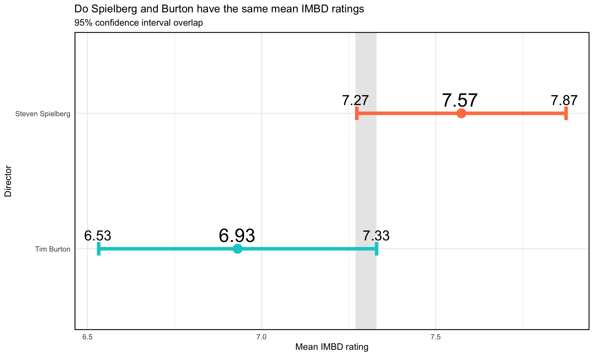

Now we conduct the mentioned t-tests:

movies_subset <- movies %>%   
  filter(director %in% (c("Steven Spielberg", "Tim Burton")))

#t-test 
t.test(rating ~ director, data=movies_subset)

## 
##  Welch Two Sample t-test
## 
## data:  rating by director
## t = 3, df = 31, p-value = 0.01
## alternative hypothesis: true difference in means between group Steven Spielberg and group Tim Burton is not equal to 0
## 95 percent confidence interval:
##  0.16 1.13
## sample estimates:
## mean in group Steven Spielberg       mean in group Tim Burton 
##                           7.57                           6.93

set.seed(1)
#t-test simulation 
obs_diff_ratings <- movies_subset %>%
  specify(rating ~ director) %>%
  calculate(stat = "diff in means", order = c("Steven Spielberg", "Tim Burton"))

null_dist <- movies_subset %>%
  # specify variables
  specify(rating ~ director) %>%
  
  # assume independence, i.e, there is no difference
  hypothesize(null = "independence") %>%
  
  # generate 1000 reps, of type "permute"
  generate(reps = 1000, type = "permute") %>%
  
  # calculate statistic of difference, namely "diff in means"
  calculate(stat = "diff in means", order = c("Steven Spielberg", "Tim Burton"))

null_dist %>% visualize() +
  shade_p_value(obs_stat = obs_diff_ratings, direction = "two-sided")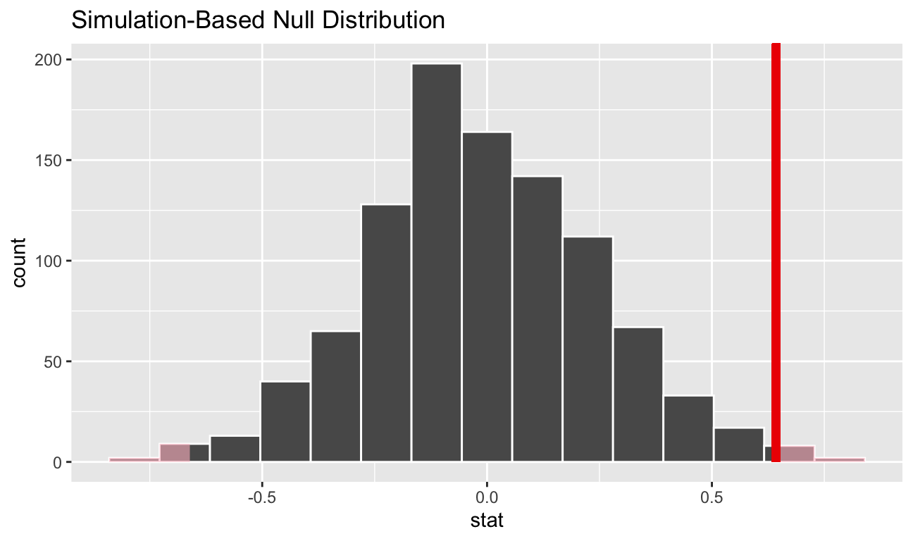

null_dist %>%
  get_p_value(obs_stat = obs_diff_ratings, direction = "two_sided")

## # A tibble: 1 × 1
##   p_value
##     <dbl>
## 1   0.012